The first part of this in-depth study of Bitcoin reveals the foundations and mechanisms of this pioneering cryptocurrency. Introduced in 2009, Bitcoin is based on blockchain, a revolutionary technology that promises security and transparency for financial transactions, without conventional intermediaries. This analysis explores the economic implications of Bitcoin, examining its price and yield, as well as key indicators such as Sharpe Ratio, Maximum DrawDown, Value at Risk (VaR), and Conditional Value at Risk (CVaR). In addition, a projection of future Bitcoin price trends will be attempted through Geometric Brownian Motion (GBM) simulation.
The next section invites us to delve into the fundamental analysis of Bitcoin, highlighting the blockchain. The aim is to decipher how this key technology guarantees the security, immutability and transparency of transactions, and its repercussions on the valuation of Bitcoin in the financial world.
The second part of this study will focus on a comparison between Bitcoin and other asset classes, assessing its contribution to portfolio diversification and its reaction to global economic changes. A more detailed analysis will enrich our understanding of financial strategies and the future potential of Bitcoin in the global economy.
Disclaimer
Please note that this analysis is for educational and informational purposes only. It is not intended as financial advice and no investment recommendation is made. The information presented in this study is based on historical data and experimental analysis, and in no way guarantees the future performance of Bitcoin or any other financial asset. Readers are encouraged to consult qualified financial and investment professionals before making any investment decisions. The author and contributors accept no responsibility for decisions made on the basis of information provided in this article.
Informations
The original language of the article is French, this is a translated version, the images and formulas are always in French and there may be other errors in the article
I. Fundamental analysis of BTC
Bitcoin, the pioneer of cryptocurrencies, stands out for its technical features and sophisticated computer architecture. Let’s delve into the intricate details of its structure and operation.
A. Technical exploration of the Bitcoin blockchain
The Bitcoin blockchain is made up of cryptographically linked blocks of transactions, forming a continuous and transparent chain of economic activity. Each block contains a set of confirmed transactions, as well as a header containing a cryptographic hash that links the block to its predecessor, thus ensuring the integrity and security of the chain.
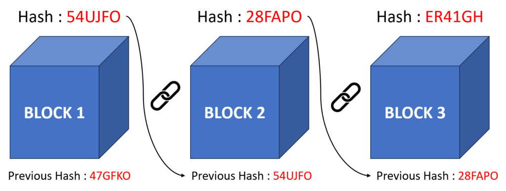
Having explored how Bitcoin transactions are secured by block hashing, the next step is to look at the validation and hashing of the blocks themselves. The heart of the Bitcoin blockchain beats to the rhythm of its consensus mechanism, which empowers participants to reach agreement on the state of the network in a decentralized manner. This consensus is achieved through a process called proof-of-work, during which miners compete to solve complex mathematical puzzles. Their successful completion enables new blocks to be validated and chained to the blockchain, reinforcing the security and integrity of the entire network.
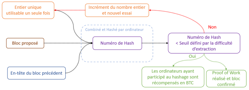
Exploring the hashing process has revealed how blocks and the transactions they contain are secured within the Bitcoin blockchain. This understanding leads to the central role of digital keys in the Bitcoin ecosystem, which are vital for the security and management of digital assets. In this system, each user is equipped with a distinct pair of cryptographic keys: the private key, which is used to securely sign transactions and attest to bitcoin ownership, and the public key, which is used to receive bitcoins and authenticate transactions.

Another key feature of Bitcoin is its limited supply. Unlike fiat currencies, which can be printed in unlimited quantities by central banks, the number of Bitcoins is capped at 21 million. This programmed limitation creates a digital scarcity that gives Bitcoin intrinsic value and makes it potentially attractive as a long-term store of value.
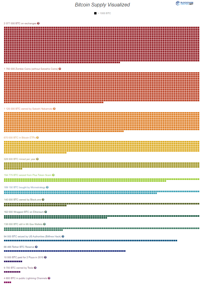
Following on from our discussion of Bitcoin’s limited supply, it is essential to consider the role of halving in this context. This mechanism, which occurs every 210,000 blocks or approximately every four years, halves the reward given to miners for each newly mined block. This process contributes directly to Bitcoin’s scarcity by progressively reducing the issuance of new Bitcoins. By mimicking the extraction of a depleting resource, halving is designed to limit supply, which can reinforce Bitcoin’s long-term value by controlling inflation.
In summary, Bitcoin’s intrinsic features, such as blockchain, limited supply, proof-of-work, digital keys and halving, form the foundation on which the Bitcoin economy rests. By understanding these fundamental concepts, we are able to fully appreciate the value and potential of Bitcoin in the modern financial landscape.
B. Economic and financial challenges
Bitcoin, beyond its status as a simple digital currency, offers a multitude of practical applications that are revolutionizing financial transactions and opening up new possibilities for individuals and businesses. These tangible use cases reflect Bitcoin’s ability to transcend the traditional boundaries of finance and meet modern needs in innovative and efficient ways.
One of Bitcoin’s most obvious applications is as an alternative store of value. In economies suffering from currency instability, Bitcoin has become a safe haven against inflation and the devaluation of fiat currencies. This feature makes it a valuable tool for individuals and companies seeking to protect the value of their wealth over the long term.
The rise of decentralized finance (DeFi) represents another significant advance in the use of Bitcoin. DeFi applications leverage blockchain technology to create financial systems that are open and accessible to all. Applications such as intermediaryless lending, decentralized exchanges (DEX) and Bitcoin-based predictive protocols offer new opportunities for investment and asset management, without the need for trusted third parties.
Beyond its practical uses, Bitcoin offers considerable economic potential that can radically transform the global financial landscape. Its growing adoption in a variety of industries testifies to its increasing relevance as a means of payment and store of value. The growing interest of institutional investors and wealth managers also testifies to its growing legitimacy as an asset class. As we explore these concrete applications and their economic potential, we are witnessing the emergence of a new financial era, driven by decentralization, accessibility and technological innovation.
II. Bitcoin’s historical performance
Since its launch in 2009, Bitcoin has transformed the financial landscape, evolving from an alternative digital currency to a major investment asset. This section examines the historical evolution of its price, volatility and risk-adjusted return, to highlight the factors that have influenced its performance over time. Through this analysis, we seek to understand the dynamics that have characterized Bitcoin and assess its potential as an element of portfolio diversification.
The data analyzed on monthly Bitcoin returns, covering the period from April 2015 to March 2024, was extracted from Investing.com. To process and visualize this data, we used : Python and specialized libraries such as Numpy, Pandas, and Matplotlib. These powerful tools enabled precise manipulation and clear representation of Bitcoin’s trends and performance over time.
A. Price and yield trends
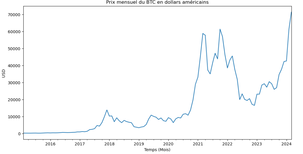
As illustrated in the chart above, the price of Bitcoin has recorded spectacular growth since 2015, climbing from $254 to $71,332. This ascent represents a staggering increase of 29,122%.
Here’s a detailed look at Bitcoin’s returns over the period studied, demonstrating not only the robustness of this digital asset, but also its ability to generate significant returns on investment despite its inherent volatility. This historical performance is essential to understanding Bitcoin’s valuation trajectory and its implications for long-term investors.
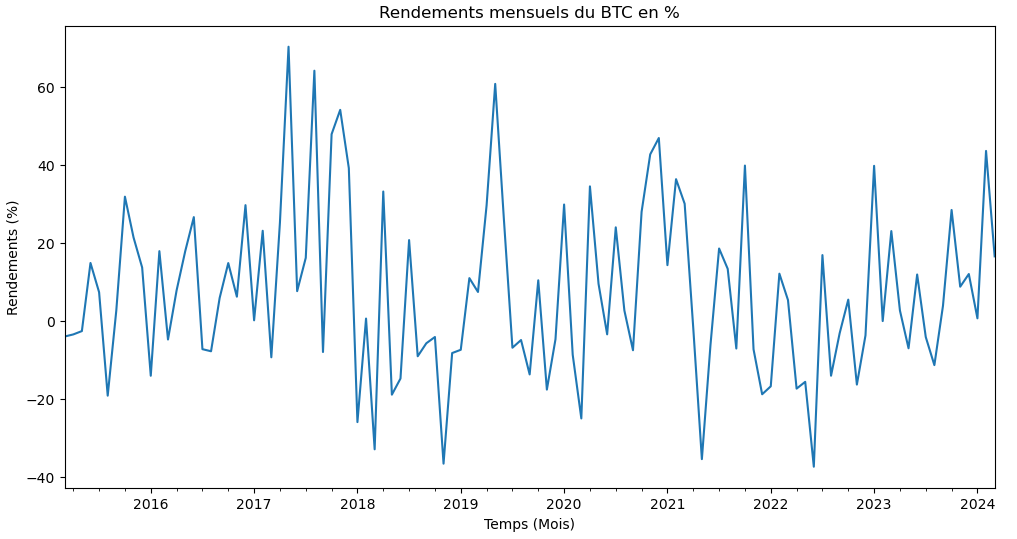
For an in-depth, quantitative analysis of this exceptional performance, we have segmented the Bitcoin study into four distinct periods:
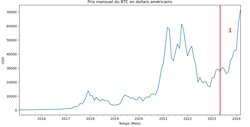
- First Period: April 2023 to March 2024, covering the last year of analyzed returns.
- Second Period: April 2021 to March 2024, covering the last three years.
- Third Period: From April 2018 to March 2024, covering the last six years.
- Fourth Period: April 2015 to March 2024, representing the full nine years of available data.
For each period, we will calculate three key performance indicators to characterize Bitcoin returns: cumulative return, average monthly return and compound annual growth rate (CAGR). This structured method enables a clear comparison of the evolution of Bitcoin’s performance over time, offering valuable insights into its growth dynamics and market trends.
A.1 / Cumulative yield
Cumulative return is an essential indicator for assessing the performance of an investment over a given period. It takes into account all gains and losses accumulated over the period, including compound interest, thus providing an overall view of the investment’s performance. This calculation is particularly useful for assessing the impact of market fluctuations on a long-term investment.
However, the cumulative return has certain drawbacks, notably its vulnerability to extreme price variations over short periods, which can sometimes give an inaccurate representation of the investment’s real performance. In addition, it does not take into account the timing of cash flows, a crucial factor for investors who make periodic contributions or withdrawals.

where ri represents the yield for period i

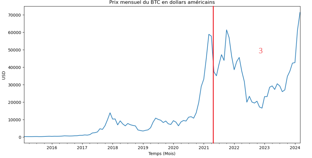
It is therefore possible to confirm that the modest returns observed during this period are attributable to a particularly high initial asset price. Indeed, when the initial investment is made at a high price level, future growth margins may be limited, thus impacting overall returns. This dynamic underlines the importance of considering the point of entry into the investment, particularly in volatile markets such as Bitcoin, where price variations can be extreme and significantly influence short- and medium-term returns.
A.2 / Average monthly yield
Average monthly yield is a measure used to assess the performance of an investment on a monthly basis, by calculating the average of price variations over this period. In addition, by analyzing the average monthly yield, investors can better assess the stability and consistency of the investment on a regular basis.
However, the disadvantages of the average monthly return include its sensitivity to extreme price variations over short periods, which can sometimes give a misleading picture of the investment’s actual performance. In addition, the average monthly return may be influenced by temporary factors or one-off events occurring during a specific month, which can make it difficult to interpret the data.

Rtotal = 9-year yield
n = number of months over the study period

Consistent with previous observations, Bitcoin’s average monthly return remains positive, testifying to the asset’s fairly robust growth. This consistency suggests a generally positive trend for investment, both in the short and long term. So, despite its notorious volatility, Bitcoin is demonstrating solid, positive returns, reinforcing its appeal as a viable investment option in the face of market fluctuations.
A.3 / Compound annual growth rate
Average Annual Growth Rate (AAGR) is a measure used to estimate the average rate of return on an investment over a given period, taking into account cumulative growth or decline over the period, as well as the effect of compound interest. This measure is particularly useful for assessing the performance of long-term investments, as it takes into account average growth or decline over the entire period.
However, CAGR also has potential drawbacks. It can sometimes give a simplified picture of an investment’s actual performance, as it does not take into account intermediate market fluctuations that can have a significant impact on overall returns. Furthermore, CAGR assumes constant growth or decline over the entire period, which may not always reflect market reality.

Vfinal = Asset value at end of 9 years
Vinitial = Asset value at start of period under review
n = number of years over the study period

BTC’s Compound Annual Growth Rate (CAGR) follows the trend of previous observations: the rate is always positive. These CAGRs show that Bitcoin has been a very successful investment over different periods. Finally, a CAGR of 87.92% for the last 9 years underlines Bitcoin’s enormous growth potential since its inception. This impressive figure shows that Bitcoin has generated extremely high returns over a relatively short period of time, attracting the attention of investors looking for exceptional returns.
Interestingly, the compound annual growth rate (CAGR) for the past year corresponds to the cumulative return over one year, a consistency that aligns with the CAGR concept. These remarkably high values reflect the ups and downs of the Bitcoin market, including periods starting at highs and ending in valleys and vice versa. The last year in particular started with relatively low prices, only to close on significantly higher levels, highlighting the volatility and dynamics of Bitcoin prices. This trend is illustrated in the following chart, demonstrating the substantial price variations over the period observed.
A.4 / Conclusion on yields
Analysis of the three types of return – cumulative return, average monthly return and Average Annual Growth Rate (AAGR) – provides a comprehensive overview of Bitcoin’s performance over different time periods. The cumulative return highlights the exponential growth in Bitcoin’s value over the long term, with impressive returns over periods of up to nine years. This demonstrates the asset’s appeal to investors seeking high returns, although it can also signal high volatility and inherent risks. The average monthly return, meanwhile, offers a more granular perspective by showing Bitcoin’s average growth on a monthly basis. This provides a better understanding of short-term trends and market volatility patterns. Finally, CAGR provides an annualized measure of Bitcoin’s average growth over different periods, highlighting its stable and sustained performance over the long term. Together, these three measures offer a comprehensive overview of Bitcoin’s performance as an investment, enabling investors to make informed decisions taking into account both the potential returns and risks associated with this dynamic crypto-currency market asset.
B. Volatility analysis
This section will focus on analyzing the historical evolution of Bitcoin’s volatility. The aim is to identify the underlying trends and patterns of this volatility, in order to provide insights into its future behavior as a potential portfolio diversification and investment tool.
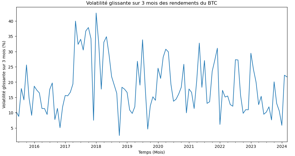
The figure above reveals the high volatility that characterized Bitcoin throughout the period analyzed. On several occasions, volatility exceeded the 35% threshold, sometimes for several consecutive months. This observation highlights the fact that Bitcoin is, by nature, a highly volatile asset, and that its fluctuations are not necessarily attributable to periods of crisis or particular events. To deepen this analysis, volatility will be examined over different time periods and annualized, providing a perspective on annual volatility over the different time intervals studied.

Xi = Individual value in dataset
X/ = Arithmetic mean of data set values
n = Total number of values

Bitcoin volatility data highlights several key trends. First, a gradual decrease in volatility is observable over time. For example, last year’s volatility was 15.46%, which is higher than previous periods. Looking in more detail, annualized volatility over the past three years is 10.94%, higher than that measured over the past six years at 8.58%, and the latter is still higher than annualized volatility over the entire nine years, which is 7.33%. This downward trend could signal a relative stabilization of this asset over time. Nevertheless, it is crucial to note that despite this decline, Bitcoin’s volatility remains significantly higher than that of traditional assets, highlighting the higher risks associated with this investment.
C. Integrated Analysis Returns/Volatility/Risk-Return
In this last section of our study, we will conduct a detailed analysis of Bitcoin’s performance by considering key aspects such as returns, volatility, and the ratio between risk and return. Our goal is to detail these elements to provide a comprehensive understanding of the dynamics of Bitcoin as an investment asset. By exploring these risk measures, we will seek to better understand the likelihood of significant losses and identify the strategies needed to mitigate the associated risks. We will begin by examining the skewness and kurtosis.
C.1 / Skewness and Kurtosis
By analyzing the distribution of Bitcoin returns, we can calculate Skewness (asymmetry) and Kurtosis (flattening). These statistical indicators will help us better understand the specific shape and characteristics of this distribution, revealing crucial details about the behavior of returns and the associated risks.

Xi = Individual value in dataset
X/ = Arithmetic mean of dataset values
n = Total number of values

Xi = Individual value in dataset
X/ = Arithmetic mean of dataset values
n = Total number of values

The analysis of skewness and kurtosis indicators of Bitcoin returns shows positive asymmetry over various periods, indicating a predominance of large positive returns over negatives. Last year in particular revealed a strongly positive asymmetry, signaling extreme gains. On flattening, three- and nine-year yields were close to normal, with a slight increase in extreme events over the past year. These observations confirm that investing in Bitcoin is marked by high volatility and an increased risk of realizing both significant gains and losses. To more accurately assess these risks, we can calculate Value at Risk (VaR) and Conditional Value at Risk (CVaR).
C.3 / VaR and CVaR
Value at Risk (VaR) and Conditional Value at Risk (CVaR) are essential risk management tools used to estimate the risk of loss in an investment portfolio. VaR measures the maximum amount of loss expected over a specific period, at a given level of confidence, thus representing the worst possible loss scenario under normal market conditions. The CVaR, or Expected Shortfall, deepens this analysis by averaging losses that occur beyond the VaR, providing a more complete view of the risks of extreme losses. These measures are particularly valuable for portfolio managers and investors, allowing them to assess and minimize potential risks in highly volatile environments like the cryptocurrency market.
The traditional VaR formula typically focuses on the average and standard deviation of returns to determine the worst-case loss scenario within a certain confidence interval. However, this approach can sometimes underestimate the risk in distributions that do not follow the Gaussian standard, especially in the presence of asymmetric returns or heavy tail distributions.

z = Quantile of the normal distribution
K = Kurtosis value
S = Skewness value

μ = Average returns over the entire period
σ = The standard deviation of returns over the period
Après le calcul de la VaR de Cornish-Fisher, la Conditional Value at Risk (CVaR), aussi connue sous le nom d’Expected Shortfall, sera déterminée en utilisant les données historiques. La CVaR est une mesure de risque qui donne une estimation de la taille moyenne des pertes qui dépassent la VaR dans les cas les plus défavorables.

α = Niveau de confiance utilisé pour la VaR (5% dans ce cas)
ri = Rendements individuels dans l’ensemble des données.
N = Nombre total de rendements qui dépassent la VaR
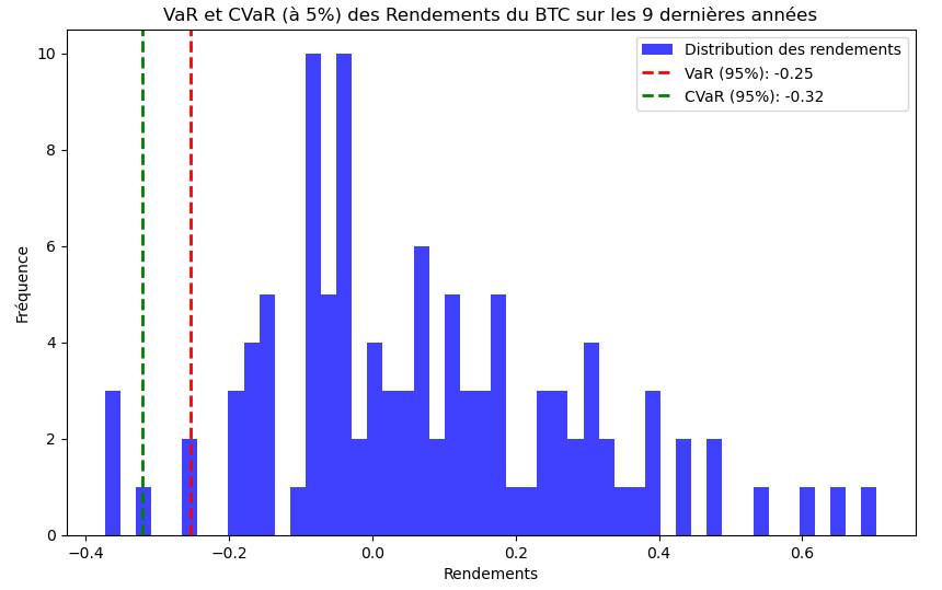
The chart above illustrates Bitcoin’s returns over the past nine years, including Value at Risk (VaR) and Conditional Value at Risk (CVaR). The VaR, set at a 95% confidence level, suggests that it is highly unlikely that the loss will exceed 25% of the value of the Bitcoin wallet. In addition, the CVaR indicates that in cases where losses exceed this VaR by 25%, the expected average loss would then be 32%. These measures provide a clear perspective on the maximum likely risk and potential losses in extreme scenarios.

For the past year, both FC VaR and CVaR are at 11%, indicating that losses have not significantly exceeded this threshold. However, over longer periods, CVaR tends to increase compared to FC VaR, reaching up to 36% for the last three years. This increase highlights that extreme losses can be more severe and the risk increases over time. In conclusion, it would be relevant to calculate the maximum loss suffered by a portfolio during this period to verify whether our VaR and CVaR models correctly estimated this maximum loss.
C.4/ Maximum Drawdown
Maximum Drawdown (MDD) is a risk measure that indicates the largest drop from a peak to a low in the value of a portfolio before it begins to recover. This is a crucial indicator to assess the maximum potential loss that the asset could suffer over a given period.

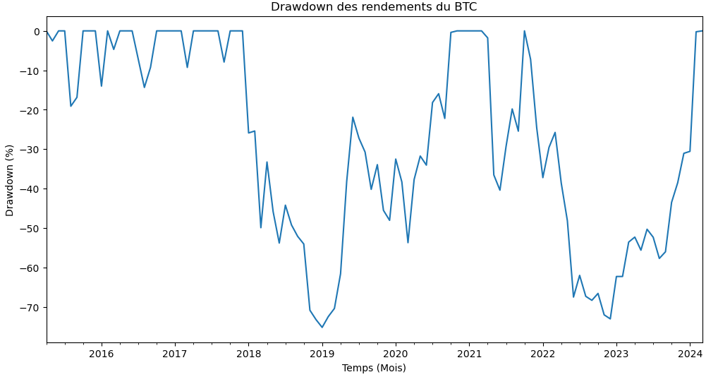

Over the past year, the Maximum Drawdown (MDD) actually corresponds to the values predicted by the VaR and CVaR of the model. However, in previous years, maximum losses of up to 73% and 75% were recorded, which represents considerable decreases. It is also observed that VaR and CVaR estimates did not anticipate such losses. This suggests that the VaR and CVaR methods significantly underestimated the actual risk of maximum loss. The Max Drawdown values reveal that the actual losses were much more severe than those projected by the VaR and CVaR models. It is therefore imperative to explore other models and understand why the variations were not fully captured. Soon, we will quantify the return per unit of risk taken by owning Bitcoin, using the Sharpe Ratio in the next part of our analysis.
C.5/ Sharpe Ratio
The Sharpe Ratio is a risk-adjusted performance measure, used to assess the effectiveness of an investment by comparing its excess return (beyond a risk-free rate) to its volatility. This ratio allows investors to understand how much additional return they receive for each unit of risk taken, helping to determine whether the additional risk taking is worth the potential returns.

Rp = Average return on investment
Rf = Risk-free rate of return (3% in this case)
σp = The volatility of investment returns

An extremely high Sharpe ratio of 9.54 indicates that Bitcoin has generated significantly higher returns compared to its volatility over the past year. This suggests an exceptional performance with a return well above the level of risk taken, which is rare and very favorable. On the other hand, for the last three years the Sharpe ratio is very low for the reasons explained previously during the presentation of the yields. Over the medium and long term, high ratios suggest that Bitcoin tends to be a profitable, though risky, investment option.
IV. Yield Cycles and Forecasts
In this section, we will explore the use of advanced analytical methods such as Rapid Fourier Transform (FFT) and geometric Brownian motion to analyze cycles and predict future Bitcoin (BTC) returns. The FFT application will allow us to break down Bitcoin price fluctuations into constituent frequencies, providing insights into underlying cycles that could influence future trends. At the same time, geometric Brownian motion will be used to simulate future BTC price trajectories, based on assumptions of price continuity and stochastic volatility. This combination of approaches aims to provide a solid foundation for understanding Bitcoin’s price dynamics and developing more informed and effective investment strategies.
A. Yield Cycles and FFT Analysis
The Rapid Fourier Transform (FFT) is a mathematical method used to analyze the frequencies composing a time signal, such as Bitcoin price fluctuations (BTC). By applying FFT to BTC price data, investors and analysts can identify periodic cycles and trends that are not immediately apparent. This analysis can help predict future price behavior by detecting recurring patterns, thus facilitating a better trading strategy based on the rhythms observed in historical price data.

Xk = The value of the DFT at the frequency index k
x[n] = n-th yield sample
N = Number of returns over the entire period
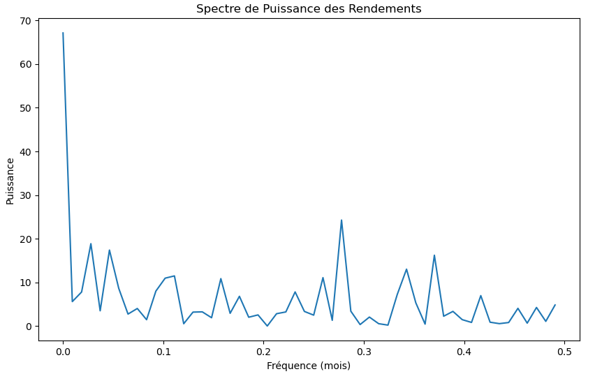
The power spectrum from the FFT on BTC yields reveals a long-term dominant cycle and several shorter cycles, as evidenced by peaks at different frequencies. The largest low-frequency peak suggests a sustained global trend or pattern in Bitcoin’s price behavior, while secondary peaks may indicate additional periodic fluctuations. For example, we may see a peak before frequency 0.3, which could indicate a cycle that repeats at that frequency. This frequency analysis can offer insights into the underlying cyclical structure of Bitcoin returns, useful for forecasting and understanding market trends.
B. Yield forecasts
The Geometric Brownian Movement (GBM) is an essential model in finance to simulate the evolution of asset prices. Although GBM generally assumes that returns follow a normal distribution, with a skewness of zero and a kurtosis of three, it remains applicable and useful even when the actual data diverges slightly from these assumptions, as is common in volatile markets such as cryptocurrencies. When skewness is moderate and kurtosis is close to three, GBM can be considered a reasonable approximation for short-term predictive analyses or simulations. By adjusting the trend (drift) and volatility parameters of the model, users can better align GBM simulations with the empirical characteristics of the data, This makes the model both practical and accurate enough for many finance applications.
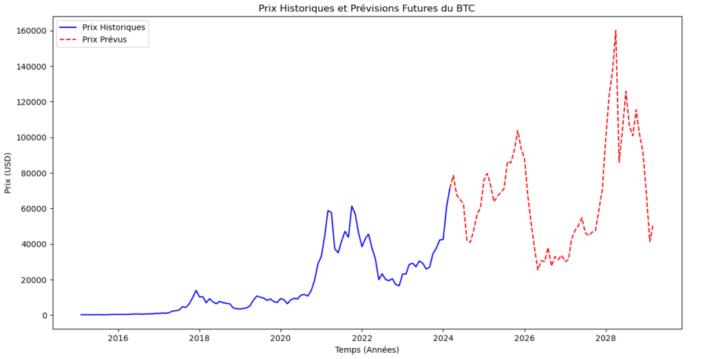
For the chart presented, the trend of Bitcoin returns was estimated using the average of logarithmic returns (60.06%) and volatility was calculated from annualized volatility (70.51%). The starting price used is the last available price in the data, $71,332. The simulation was projected over a 5-year period, which represents a significant duration given the initial 9-year database and the highly volatile nature of Bitcoin. Although only one scenario has been calculated for this illustration, it is possible to extend this forecast to 5.50, or even 500 different scenarios to explore various potential future Bitcoin price trajectories. This approach provides a broader view of possible price changes under different market conditions.
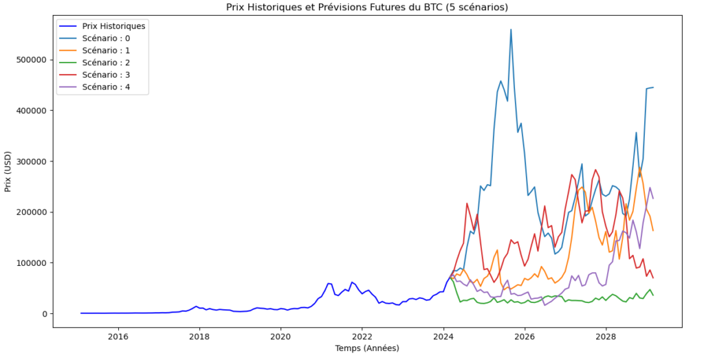
Accurately predicting the future prices of Bitcoin is extremely difficult, if not impossible. For a clear visualization, considering 5 scenarios makes it easy to observe the final values of each simulation. However, for a larger number of scenarios, it would be wise to display the yield distribution next to the main chart. This method allows a better understanding of the variability of the possible results and a graphical representation of the dispersion of the expected returns, which enriches the analysis of risks and opportunities.
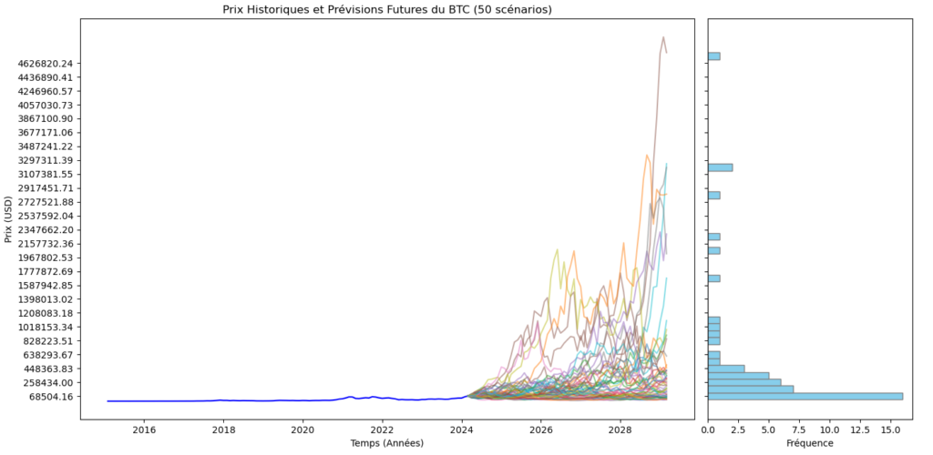
Indeed, although the use of a histogram facilitates the visualization of the price distribution, the volatility of Bitcoin can lead to the presence of outliers that mask the actual concentration of returns. To overcome this problem, especially in the case of simulations extended to 500 scenarios, the adoption of a logarithmic scale is recommended. This approach makes it possible to better represent the dispersion of values, making the extreme data more manageable and highlighting the areas of concentration of yields, for a more precise and informative analysis.
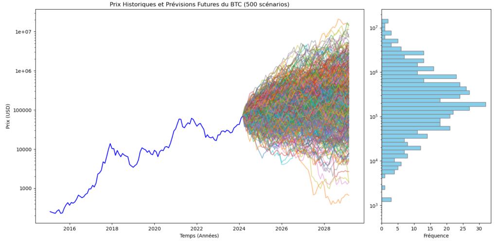
Using the logarithmic scale, presents a simulation of 500 prediction scenarios for Bitcoin, next to the corresponding histogram. This scale makes it possible to better observe the results of the simulations, in particular by making outliers more visible and by detailing the concentration of yields. The logarithmic scale widens the perspective and clearly reveals the distribution of final prices, including extreme events. It also confirms the unpredictability of Bitcoin and the wide range of possible outcomes, highlighting once again the speculative nature of the asset.
Conclusion
In summary, our in-depth exploration of Bitcoin has revealed a cryptocurrency that stands out both for its underlying technology and its behavior as a financial asset. Through the mechanisms of blockchain, we have discovered a system of secure and transparent transactions that challenges the traditional paradigms of finance. The economic implications are considerable, notably due to the limited supply of Bitcoin which makes it a potentially attractive store of value, not to mention its growing influence in the decentralized finance universe.
The performance, volatility, and risk ratios analyses highlighted the exceptional performance but also the inherent volatility of Bitcoin. The analysis showed that, despite significant volatility, Bitcoin has recorded considerable gains over the long term. However, traditional tools such as Value at Risk and Conditional Value at Risk can underestimate risk in such unpredictable markets. Simulation scenarios based on the Geometric Brownian Movement (GBM) have made it possible to project potential future trajectories of Bitcoin, despite the limitations inherent in any attempt to predict financial markets.
In conclusion, Bitcoin, armed with its revolutionary blockchain technology and its meteoric growth trajectory, presents both opportunities and challenges for investors. Understanding the nuances of its volatility and the calculation of its risk-adjusted performance remains crucial to navigate this dynamic investment space.
As we complete this first part, our analysis of Bitcoin will continue. The second part of the article will focus on a comparison between Bitcoin and other asset classes, an investigation of its role in portfolio diversification and an examination of its reactions to major global economic trends.

Laisser un commentaire